Examples
Example 1: Simple Heating System
Case study with a simple heating system SimpleHeatingSystem.mo built in Modelica.
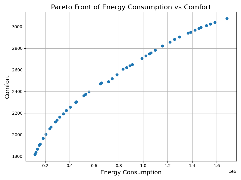
The idea is to heat a room, when the room heats faster, human beings feel more comfortable, but the energy consumption and cost become higher. The heating power and target temperature should be optimized to find the trade-off between human comfort and energy consumption.
| Parameters | Objectives |
|---|---|
| Heating Power | Human Comfort |
| Target Temperature | Energy Consumption |
| Goal | |
| Maximize Human Comfort Minimize Energy Consumption | |
I. Generate Feature Tree/Model from A Modelica File (Optional)
Step 1: Generate the parser code using ANTLR4
antlr4 -Dlanguage=Python3 modelica.g4
Some files have been generated, e.g.:
modelicaLexer.pymodelicaParser.pymodelicaListener.py
Step 2: Configuration
configure parse_modelica.py
# Configuration
file_name = 'SimpleHeatingSystem.mo'
configure feature_model.py
# Configuration
model_name = 'SimpleHeatingSystem.mo'
output_file = 'feature_model.json'
include_equations = True  # set to "False" if equations should be excluded
Step 3: Parse the Modelica model and generate the feature tree
python feature_model.py
You will see the result in the terminal:
SimpleHeatingSystem
├── parameter Real (Q_max)
│   └── value=5000
...
│   └── value=()
├── Boolean (heater_on)
│   └── value=()
├── constant Real (c_p)
│   └── value=1005
...
├── Equation 1: der(T_room)=(Q_heat*efficiency-(T_room-273.15))/(m_air*c_p)
...
└── Equation 7: der(comfort)=ifheater_onthenefficiency*Q_heat/(accumulated_discomfort+1)else0
The feature model will be then saved as feature_model.json:
{
    "name": "SimpleHeatingSystem",
    "children": [
        {
            "name": "parameter Real (Q_max)",
            "children": [
                {
                    "name": "value=5000",
                    "children": []
                }
            ]
        },

        ...

        {
            "name": "Real (Q_heat)",
            "children": []
        },

        ...

        {
            "name": "Boolean (heater_on)",
            "children": [
                {
                    "name": "value=()",
                    "children": []
                }
            ]
        },
        {
            "name": "constant Real (c_p)",
            "children": [
                {
                    "name": "value=1005",
                    "children": []
                }
            ]
        },

        ...

        {
            "name": "Equation 1: der(T_room)=(Q_heat*efficiency-(T_room-273.15))/(m_air*c_p)",
            "children": []
        },
		...

        {
            "name": "Equation 7: der(comfort)=ifheater_onthenefficiency*Q_heat/(accumulated_discomfort+1)else0",
            "children": []
        }
    ]
}
II. Run Optimization
Step 1: Configure global settings for the optimization
# Basic settings
"MODEL_NAME": "SimpleHeatingSystem",
"MODEL_FILE": "SimpleHeatingSystem.mo",
"SIMULATION_STOP_TIME": 3000,  # in seconds

# Results precision
"PRECISION": 2,  # decimal places

"PARAMETERS": ["Q_max", "T_set"]
"OBJECTIVES": [
    {"name": "energy", "maximize": false},
    {"name": "comfort", "maximize": true}
],

"PARAM_BOUNDS": {
    "Q_max": {
        "bounds": [1000, 5000],
        "type": "float"
    },
    "T_set": {
        "bounds": [280, 310],
        "type": "int"
    }
},

"OPTIMIZATION_CONFIG": {
    "USE_SINGLE_OBJECTIVE": false,
    "ALGORITHM_NAME": "nsga2",
    "POP_SIZE": 5,
    "N_GEN": 1
},

"PLOT_CONFIG": {
    "PLOT_X": "Energy Consumption",
    "PLOT_Y": "Comfort",
    "PLOT_TITLE": "Pareto Front of Energy Consumption vs Comfort",
    "ENABLE_PLOT": false
},

# import libraries that the model needs
"LIBRARY_CONFIG": {
    "LOAD_LIBRARIES": false,
    "LIBRARIES": [
        {"name": "", "path": ""}
    ]
},

# Parallel computing
"N_JOBS": -1  # Options: '-1', '1', 'n', 'None'
Step 2: Run Python script: python optimize_main.py
You will see
- the models have been loaded in different workers for parallel computing
- parameters have been set for different models
- simulated results of each model
like this:
Number of variables: 2
Lower bounds: [1000  280]
Upper bounds: [5000  310]

Load model result in worker: True
Load model result in worker: True
Load model result in worker: True
Load model result in worker: True
Load model result in worker: True

Parameters set: {'Q_max': 4173.26, 'T_set': 284.49}
Parameters set: {'Q_max': 1220.76, 'T_set': 305.78}
Parameters set: {'Q_max': 1951.81, 'T_set': 299.48}
Parameters set: {'Q_max': 4675.92, 'T_set': 289.72}
Parameters set: {'Q_max': 2044.53, 'T_set': 305.47}

...
The simulation is running:
Simulation results: {'energy': 344482.35, 'comfort': 1873.97}
OMC session closed successfully.
Simulation results: {'energy': 1490363.54, 'comfort': 836.97}
OMC session closed successfully.
Simulation results: {'energy': 608112.5, 'comfort': 2298.91}
OMC session closed successfully.
Simulation results: {'energy': 1158015.95, 'comfort': 1213.1}
OMC session closed successfully.
Simulation results: {'energy': 778781.79, 'comfort': 1521.05}
OMC session closed successfully.
...
You will see the results at the end of the simulation like this:
...
| 100 | 5000 | 50 | 0.0031202395 | f |
Optimization Results:
Solution 0: Energy = 1683944.96, Comfort = 3074.81,
Solution 1: Energy = 118249.77, Comfort = 1817.60,
Solution 2: Energy = 1683944.96, Comfort = 3074.81,
...
Solution 47: Energy = 298007.19, Comfort = 2135.79,
Solution 48: Energy = 1064447.73, Comfort = 2758.86,
Solution 49: Energy = 319668.29, Comfort = 2162.22,
After that, you will see the Pareto front:
Example 2: Electric Driving Robot
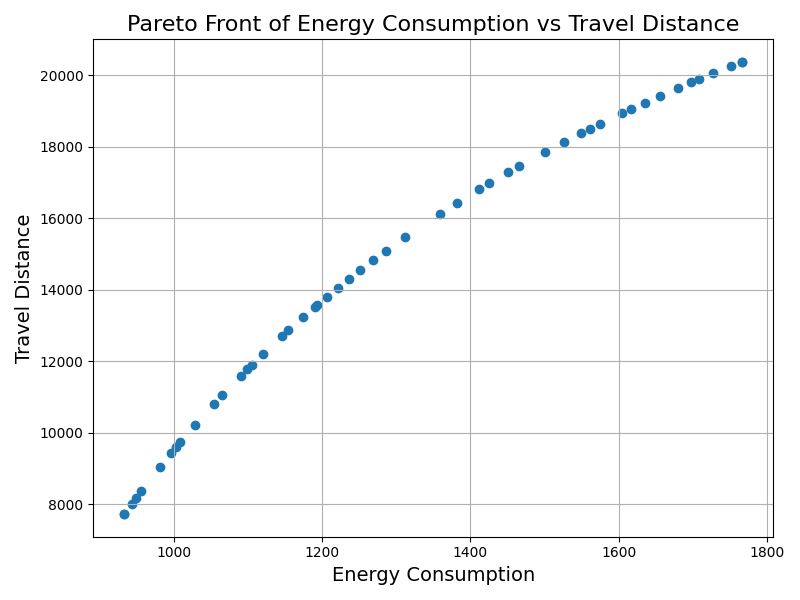
Case study with an electric driving robot built in Modelica.
The robot should optimize its driving speed to find the trade-off between driving distance and energy consumption.
| Parameter | Objectives |
|---|---|
| Driving Speed | Travel Distance |
| Energy Consumption | |
| Goal | |
| Maximize Travel Distance Minimize Energy Consumption | |
Configurations in config.py have been modified accordingly.
After the optimization, the Pareto front will show:
3. Electric Car-sharing Systems
The system should optimize its number of cars which feeds into the system to find the minimized total waiting time (when the user comes, if no cars are available, the user waits for a while, then the user gets a car if it is available or the user leaves without getting a car) and total charging time.
| Parameter | Objectives |
|---|---|
| Number of Cars | Total Waiting Time |
| Total Charging Time | |
| Goal | |
| Minimize Total Waiting Time Minimize Total Charging Time | |